Designing Machine Learning Systems for High Velocity Trading

As one of my works at Mu Sigma Labs, I was part of a research project on the High Velocity Time Series on early 2019. One of the goals was to create a high velocity trading app using Pair Trading.

The Requisite terms

Long and Short trades

Long trades are buying a security. Short is selling a security even when you don’t own it. It generally means that you are borrowing someone’s securities and selling them in the hopes of buying it back for lower cost later and returning it and hence, making a profit. You don’t really have to do it though; exchanges take care of it and let you sell when you don’t own a security.

Pair Trading

The idea of pair trading is to find matching securities that behave similarly and trade when they diverge on the basis that they’ll eventually revert and come back together.

Let’s take a toy example of two stocks A and B

Once you have a good pair security and detect a divergence then the simple strategy is to short the security that is up, long the one that is down.

How does it work?

Let’s say securities A and B diverge like this So you short A and long B.

Let’s see how revert can happen after a pair diverges.

1. A might be misbehaving, and A comes back down. In this case, since you shorted A, you end up making profit when it goes down and there is little change in B so no loss there. So, in total you are in profit.
2. B might be misbehaving, and B comes back up In this case, since you longed B, you end up making profit when B goes up. And there is little change in A so no loss there. So, in total you are in profit.
3. Both might be misbehaving, and they meet in the middle In this case, you make some profit on A when it goes down due to short and make profit again on B when it goes up. Again, in total you are in profit.

These are ideal cases. Most of the time you get a mixture of these, but if the securities are indeed a pair and you detected divergence correctly and within time, you’ll always make profit in an ideal world.

A pair

Let’s define what it is to be a pair a bit more. A straightforward way to think about a pair would be correlated series. The examples above showed positively correlated securities, though that is not necessary. A negatively correlated series would work just as well. You’ll just change the long, short choices. And the pair need not have similar values. You can just buy or sell weighted amounts based on their value. For example, if security A is 5X the value of B historically you can buy/sell 5X the amount of B for every 1X of A.

Co-Integration

Correlation is just one of the ways to define a pair. Another way is to use Co-Integration. Co-Integration is a statistical measure of distance between the two series is stable over time. If the distance is stable over time, then the series’ are said to be co-integrated. So, if they move apart, they’ll eventually come back together.

You can think of co-integration as a more general form of correlation. For example, let’s say you are tracking two objects moving, the location and velocity might seem uncorrelated, but the acceleration might be related. So, co-integration can detect these kinds of relationships.

The System

We wanted to build a system that would automate the process of finding pairs, detecting divergence, figuring out the amount and executing trades. The system would have to do all that in realtime.

Basic Architecture of the system is as follows: 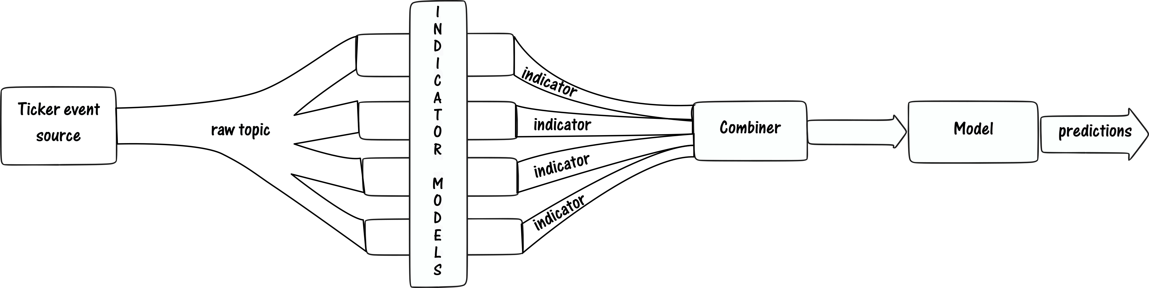Raw ticker is not enough to make these decisions, so there’ll be some real time feature engineering required. The features/indicators could be anything like OHLC values over a period, Hurst exponent, even social media indicators, etc. The model finally will be consuming the features and outputting the trades. All these are streaming components. We chose Kafka as the backbone of the system since most of our infra was self-hosted. The Kafka was also sink-ed into a InfluxDB to be able reference any historical values. The execution of trades was done by a separate service that would connect to a broker gateway and execute them.

Systems like this require a lot of experimentation. Features and models will be experimented on. Our focus was to make fast iterations on these. So, we built abstractions/libraries for building these realtime jobs. Data Scientists can write the job in a single file of R/Python, the job abstraction takes care of listening, writing to Kafka, writing to DBs, etc. Abstractions are essential for fast experimentation in data science because they allow data scientists to quickly create prototypes and test new ideas without having to rewrite existing code. They also allow developers to quickly make changes to existing code without having to understand the underlying complexity of the system.

A general structure of the ML (Machine Learning) job would be as follows:

def setup():
    # setup code
    # this is run once when the job starts
    # this is where you can setup DB connections etc
def process(data: dict) -> dict:
    # process code
    # this is run for every message on kafka
    # data is the message
    # this is where you can do your processing
def recover():
    # recover code
    # this is run when the job is recovering from a restart

Similarly in R

setup <- function() {
    # setup code
    # this is run once when the job starts
    # this is where you can setup DB connections etc
}
process <- function(data) {
    # process code
    # this is run for every message on kafka
    # data is the message
    # this is where you can do your processing
}
recover <- function() {
    # recover code
    # this is run when the job is recovering from a restart
}

This combined with a bunch of helper functions to read/write DBs etc. made it easy to write ML jobs. These jobs would then be wrapped in Java (which was doing things like listening to Kafka etc.) and built into a docker image by our CI system that were deployed on Kubernetes. All these jobs would be horizontally scalable based on how many tickers we wanted to process.

To combine all the features into a single topic for consumption by downstream model or in some cases a second order feature engineering we used Apache Spark Structured Streaming. The spark job would read from multiple topics specified in a config and basis the timestamps would perform a streaming join on all the inputs and produce a single output topic.

These were all hooked up to a nice little web app built with NodeJS, Angular, WebSockets for monitoring and controlling the system.

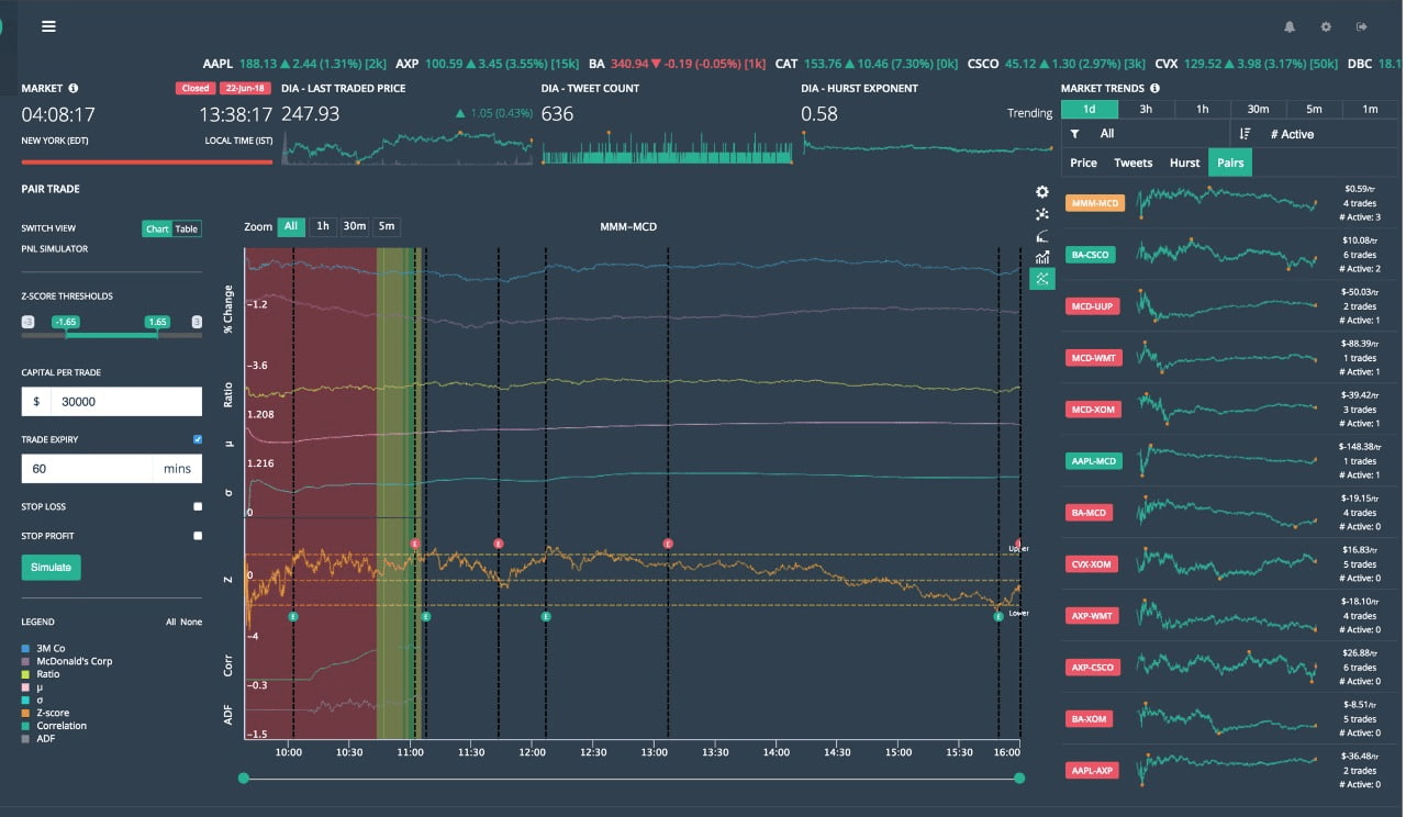
We showed the system could be run profitably (modestly) on a small set of tickers (100) in paper trading.

Further Improvements

This system works well when you have one or few models predicting for all pairs of tickers but if we split the models for each pair then the number of deployments would quickly explode (for example, if we have 1000 tickers then we would have 1000*1000 models (= number of possible pairs)). We partially supported this by running the pair level models only if there’s some evidence from the indicators that two tickers could be pairs. This was done by a separate orchestrator service that would listen to the indicators and trigger the pair level models. But it’s still not scalable enough for if we wanted to support all tickers. One of the alternative architectures we explored was to use Akka to build each pair model as an actor and have a separate actor that would listen to the indicators and trigger the pair level actors. This would allow us to scale to any number of tickers.